Lunar Gravity Models and a Lesson in Humility

My current work project has involved performing some fascinating and really hard math and modelling work for Goddard Space Flight Center, in support of the potential BOLAS mission. This has entailed diving into a codebase written primarily from 1990-1993, giving it a facelift, and expanding it’s functionality. The whole “legacy code” part of my trip into this codebase could and probably will make up an entire post of it’s own someday, but for this post I’ll primarily be talking about the gravity model we’re using, how I built and iterated upon it, why we’re studying the moon with a tethered spacecraft, and finishing with a recent and thoroughly eviscerating (for me, of course) lesson in humility.

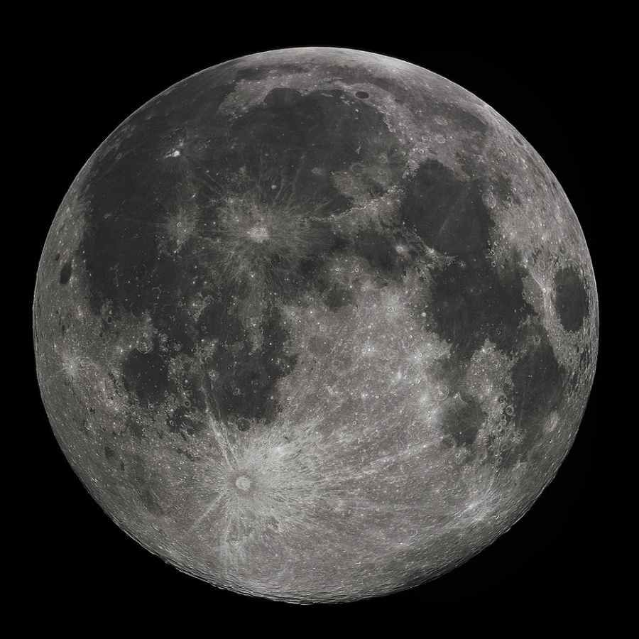
The Lunar Gravity field

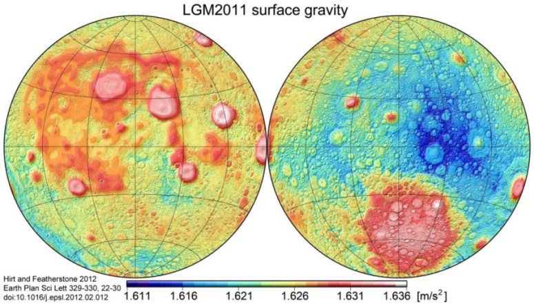
… is sorta kinda weird. As in really weird. It was known shortly before the Apollo missions that things weren’t quite “right” after anaylsis of the Lunar Orbiter tracking data - itself a sort of navigation test to prepare for the upcoming Apollo missions. It was understood then that the largest anomalies were due to mass concentrations on the Lunar maria, and this does make some degree of sense. These regions are primarily made of very dense (relative to most of the lunar regolith) basaltic lava.

Interestingly, the moon’s geometric center and center-of-mass are not the same: the center of mass is ~2 kilometers closer to the Earth

However, this alone can not describe the magnitude of the anomalies. So the composition of these regions is only part of the answer, and the rest is up for debate and discovery. We do, however, know enough to build an accurate model allowing us to compute accurate trajectories for low-lunar orbits.

Astrodynamic Models, or, “close enough”

It might seem that absolute precision is required to implement feasible models for computing spacecraft trajectories - but that’s only partially correct. There’s a balance between computability (or at least, the speed at which computations proceed) and the obvious need for accuracy since an incorrect trajectory differing only in meters could potentially spell disaster for a mission.

But the amount of factors one must consider when computing a trajectory are rather dazzling, as we can include:

• solar pressure, or the force of the solar wind on sunward elements of a spacecraft
• minute atmospheric drag forces - even the space station, for example, experiences some atmospheric drag at it’s altitude in LEO
• as an additional note on the above, the sun’s relative activity level can also cause the thermosphere to expand, increasing atmospheric drag
• drag due to the local magnetic field, itself also affected by the sun
• tidal effects, due to the shifting of mass with the tides
• even the lower-atmospheric tides have recently been added to models!
• in the case of tethered spacecraft, the temperature of the Tether changing the tether material’s properties also affects orbit propagation
• n-body perturbation effects - e.g, the Moon for objects in LEO, or most of the solar system for craft in deep space
• and of course, the gravity field of the primary body influencing the simulation

If you’d like to read more on the complex topics of atmospheric drag (it’s kinda fascinating!), I found this excellent presentation while verifying things I’ve written in this article. Clearly, though, modelling a trajectory is going to require quite a bit of computation and careful inclusion of myriad external influences.

Because of this complexity, though, it’s not really possible to compute an exact trajectory for any mission. Often, “close enough” is more than good enough as most spacecraft will feature maneuvering thrusters. In the case of satellites only living in LEO with no maneuvering abilities, they benefit from our experience in modelling Low-Earth orbits and usually are given orbits that will last throughout their mission lifetime.

We can make simplifying assumptions and adjustments to our models though, usually based on the mission requirements or the particular bodies the mission is focusing on. In the case of my work, we don’t have to worry about magnetospheric, ionospheric, atmospheric, etc sources of drag. Tidal effects also aren’t a consideration we need. Things like solar pressure can be discarded after a bit of thought (at least for initial models), as it’s likely the lunar gravity field is going to be much more chaotic and much more important to consider than the effects of solar pressure (also, we’re using a thin rope tied between two 3U cubesats - not a huge area for solar pressure to act upon).

So our primary considerations become the gravity field, a tiny contribution from Earth’s tug on a lunar satellite, and a whole bunch of work relating to the dynamics of tethered spacecraft.

“Nonspherical Gravitational Perturbation Model”

Or, translated from a wicked complex (but useful) document published by Goddard - how to model the gravity field of nonspherical bodies (most of them) and account for their own unique mass-density anomalies in said model. A copy of the Goddard document I’m currently referencing can be found here, for those so inclined to cause what is probably just short of mental self-harm.

Unsurprisingly, most of the planets and moons in the solar system aren’t really that close to being perfectly spherical. Besides that, they too have non-uniform densities throughout their interiors. The Earth isn’t just somewhat oblong - there’s also a higher density region just under the crust (in the mantle) near the equator.

In Martian models, consideration is given (via extra parameters) to seasonal variations in mass-density at the poles caused by the sublimation-condensation cycle of carbon dioxide at the Martian poles

These various anomalies in gravity fields have resulted in most models using spherical harmonics. This contrasts with what most people learn and use in highschool physics for calculating gravitational forces:

\begin{equation} F_{g}=\frac{Gm_{1}m_{2}}{r^{2}} \end{equation}

This point mass model works fine for most situations, and certainly suffices for mathematics and physics in school. But it’s only used in astrodynamics when the conditions are apt for it’s use - in particular, if a body is far enough away that the minute changes and pertubations in it’s gravitational field wouldn’t be a factor anyways.

So we use models that can accomodate this - or “Nonspherical Gravitational Perturbation Models” in the document linked in the first paragraph of this section. Spherical harmonics do this by breaking down mostly-spherical bodies into subregions, overwhich we calculate small additional contributions to our crafts acceleration vector per subregion. As far as I understand it (and do correct me if I’m wrong), it’s like integrating the mass-density over the sphere. Spherical harmonics are an approximation though, so we use summation notation:

\begin{equation} A_{G} = \frac{\mu}{r} + \sum_{n = 2}^{N} \sum_{m = 0}^{N}(P_{n}^{m}sin\theta)(C_{n}^{m}cos(m\varphi) + S_{n}^{m}sin(m\varphi)) \end{equation}

An important note is that we actually do still use that simplified formula we mentioned earlier. That’s the base quantity of gravitational force we can expect to find around a body, and that doesn’t really change much. The spherical harmonic quantites help us fine-tune our calculations to account for the minor variations in mass-density of most planetary bodies, and accounting for these minor changes is extremely important in the case of the moon as it has so many variations (some of which really are not that minor at all). Let’s break down this equation a bit more, though.

Spherical Harmonic Geopotential models

\begin{equation} A_{G} = \frac{\mu}{r} + \sum_{n = 2}^{N} \sum_{m = 0}^{N}(P_{n}^{m}sin\theta)(C_{n}^{m}cos(m\varphi) + S_{n}^{m}sin(m\varphi)) \end{equation}

Trust me, that first burst of fear over “oh god what is this math” doesn’t go away. Any sudden feelings of imposter syndrome you may or may not feel as a person without their degree working with people with PhD’s doing math like this though… well, that does fade over time. A little.

But we can break this model down into digestible chunks. Let’s start with the easiest bits- the degree and order, \(n\) and \(m\). In the case of our gravitational models, the high limit is going to be set by the available Stoke’s coefficients and to what degree and order those go out to (onto those next!). We will also commonly choose a limit of our own - commonly below our max - to balance the speed at which the simulation runs with the requisite accuracy. What makes this choice so important is how the max degree and order cause the required number of calculations to grow non-linearly. Lets say we’re going to calculate the above equation for a max \(N\) of 50 - once we get to \(n = 50\), we have to restart with \(m = 0\)… and iterate \(m\) all the way up to 50, recalculating much of our math at each step. And once \(n\) steps again, we start that all over.

\(C_{n}^{m}\) and \(S_{n}^{m}\) represent what are called (as far as I know, going off various papers) “Stokes Coefficients”. These are values that are calculated using various experiments, usually long-duration gravimetry missions. In the case of the moon, this was the GRAIL mission, which was based heavily on the GRACE mission. Both performed gravimetry measurements that generated large tables of coefficient data (the NASA database of these constants, for several bodies, can be found here).

In the case of the moon, the data tables go out to degree and order 900 - a rather tremendous improvement over previous models. My current work maxes out at order and degree 270, as that is already 36,000+ lines of coefficient data to read in from a file, and then to store in RAM (and also to facilitate fast access to from multiple threads…). The coefficients are then retrieved by indexing into these tables for a given \(n\) and \(m\) and retrieving the relevant coefficients.

\(cos(m\varphi)\) and \(sin(m\varphi)\) are part of that core inner loop - here, \(\varphi\) represents the lattitude of our satellite expressed in body-fixed coordinates (body-fixed meaning that if we’re around the moon, our measurements are all done relative to a non-rotating frame fixed on the moon). \(sin(\theta)\) is the \(sin\) of our longitude in turn, and our last measurement \(r\) is used in the outermost calculation (done only once). This simply represents the radial distance of our body from the center of our influencing body (unsurprisingly). These variables are all fairly easily calculated from the conventional (x,y,z) cartesian coordinates we work with elsewhere in our simulation, however.

The last major element of note is \(P_{n}^{m}\), representing the “associated Legendere polynomial”. This is where my lack of (complete, at least) college education really begins to show but I’ll attempt to do my best at explaining how this works. Effectively, this equation occurs when solving Laplace’s equation in spherical coordinates - Laplace’s equation often comes up in this field as it can be used to accurately describe the behavior of gravitational potential fields, particularly in relation to their “shape”.

The associated Legendere polynomials are the canonical (somewhat akin to “standardized”) solutions of the Legendere polynomials, in particular relating a degree and order value to their solutions and the fact that they can rather perfectly describe the solution to partial differential equations taken along the surface of a sphere.

We use those to help us find the small mass-density variations that affect our final geopotential result, and since we’re iterating through a spherical harmonic series of variying degree/order, increasing the degree and order just results in us taking more and more infitisemal chunks of the body in question. Its like a “detail” level, so-to-speak.

Humility

Oh, good lord was this an evisceration for me. At the end of the day, though, it’s definitely more of a good thing - it’s for the best that I am more self-critical of my own math code. Especially given that linear algebra was my worst math subject in University (differential equations, I loved those… matrices, no). The previous matrix class in my work software was clearly written by a scientist - meaning that, by god, it works and is mathematically sound. But it could use some cleanup.

In this matrix object, the data was stored in a “jagged” array as m_data[150][150]. Jagged arrays aren’t great because they fragment the memory and make things physically less cohesive in-memory - meaning it’s harder for the CPU to just consume a whole row or chunk of the data at once, instead forcing it to gather the data from disparate locations. This can really add up, and profiling runs had already highlighted it as rather bad for our CPU.

So I replaced the index-from-1 logic with the conventional (for C++!) logic of indexing from 0. Then, I replaced the old data storage method with a single array that holds all the elements for our (Rows,Columns) sized vector. I rewrote our math operators (how we do +, -, * between matrices) to use references, standard-library functions, and to be a bit faster in some cases (in detail: I wrote a few SIMD algorithms for things like matrix transposes).

But in writing this math, I didn’t think very critically about it or think to double check my math code. Mistake 1. Mistake 2 was writing such a vital class and not writing unit tests for it - something I’ve been meaning to get better about. To make it worse, the unit tests could have been very simple to write and would have absolutely found all my issues.

Sometime a few weeks ago, the math that uses these matrices the most seemed to be exploding and just not acting right. Instead of assuming immediately that it was the newly added matrix class to otherwise functional code that broke things, I assumed it was many things besides my matrix class. I did end up identifying other bugs - but they weren’t the bug(s) causing the issues, just things that had luckily not had any major side effects yet. So I kept searching - and the closest I got to questioning my work was that I made an error converting from the index-from-1 format. Despite finding a few instances where I did actually perform that incorrectly, it still didn’t fix the issue.

Then I re-examined my Matrix-Vector multiplication (i.e, Matrix<Rows,Cols>*Vector<Rows>). Oh, no:

// code edited from actual source for size, privacy
Vector operator*(const Matrix& mtx, const Vector& vec) {
    Vector result;
    for (size_t i = 0; i < Cols; ++i) {
        for (size_t j = 0; j < Rows; ++j) {
            double sum = 0.0;
            for (size_t k = 0; k < Cols; ++k) {
                sum += mtx.GetElement(i, j) * vec[k];
            }
            result[j] = sum;
        }
    }
    return result;
}

This is not even close to correct. I don’t actually know what this would even do, to be honest. For one thing, it starts out fundamentally broken - all my math did! I was repeatedly using i as the Column index, looping from 0 to num_columns. Really, i represents the rows and the range should’ve been to num_rows. So that’s already broken. But the math itself is also fundamentally broken - multiplying a Matrix by a vector is a rather simple operation, in the end. The output will be a vector, and the math itself could be seen as breaking each row of the matrix down into a vector - and performing the dot product of the matrix sub-vector with the input vector.

The correct math is much simpler, and trust me - I’ve tested this math:

Vector operator*(const Matrix& mtx, const Vector& vec) {
    Vector result;
    for (size_t i = 0; i < Rows; ++i) {
        result[i] = 0.0;
        // Take the product of mtx's row "i" and the Vector "vec"
        for (size_t j = 0; j < Cols; ++j) {
            result[i] += mtx.GetElement(i, j) * vec[j];
        }
    }
    return result;
}

I remember sitting at my desk that day a few weeks ago thinking “Well, shit”. I hadn’t wasted a week of debugging, entirely - there were still legitimate issues I fixed. But timelines are tight, and I could’ve fixed the root cause far sooner and moved on if I had

• reflected more on my own code
• tested my own code
• not let my confidence go entirely to my head

I spent the rest of that day going through my math code, double checking it rigorously. And I actually did fix a few things, to be honest. It was an important lesson and it’s still a bit painful to think about - no one likes being punched right in the ego. But at the end of the day, it’ll make me a better programmer if I’m more able to truthfully assess my own work. And if I can accept my own mistakes - like this whole debacle.